
Sparse principal component analysis in cancer research
Background
Recent modern technologies have advanced cancer research with new discoveries (1-14). These new technologies, such as genomic data and image data, often generate huge amount of information; however, analysis of such big data has not been straightforward. Principal component analysis (PCA) is one common approach to deal with the high-dimensional data by reducing data dimension into a manageable and analyzable scale. The PCA has shared many fruitful stories in cancer research in terms of genomic profiling discoveries and personalized medicine (1-7). For example, in gene microarray data analysis, Khan et al. (3) tried to use gene expression data to classify patients with the small, round blue cell tumors into several subgroups for specific treatments. Their approach first applied PCA to reduce data dimensionality. The resulting 10 PCA components were then used for analysis of artificial neural network which later correctly classified disease subtypes and identified the genes most associated with the subgroups. Similarly, Pomeroy et al. (6) used PCA to reduce gene expression data into three PCA components which were able to separates brain tumors from normal brain tissues, as well as to distinguish various brain tumor subtypes. In addition, Chen et al. (7) utilized PCA to derive a risk index score for various gene signatures in different cancers to evaluate prognostic and predictive values of the signatures. In the analysis of single nucleotide polymorphisms (SNPs), population stratification is often used to control for systematic ancestry differences in genome-wide association studies, but it could generate false associations. To detect and correct population stratification, Price et al. (5) employed PCA to minimize spurious associations while maximizing power to detect true associations. By using this approach, Hunter et al. (4) discovered four SNPs with risk of sporadic postmenopausal breast cancer in a genome-wide association study. In image analysis, Seierstad et al. (2) used PCA to summarize massive data generated from magnetic resonance spectroscopy. The resulting reduced data (PCA components) were able to separate clusters of the different xenografts and rectal cancer biopsies and to reflect underlying differences in metabolite composition.
While enjoying successful use, one drawback in PCA limits its broad application. That is, PCA reduces data into a lower dimension space, called principal components (PCs), to mimic the original data. The 1st PC explains the maximum of total variation, the 2nd PC explains the 2nd largest variation, and so on. Each PC is a weighted average of all variables (e.g., genes or image features) with a weight (called loading coefficient) assigned to each variable. This formula raises a serious concern that if a variable is a noise (meaning no true effect in the model), would it be better to exclude the variable during constructing PCs so that they become more robust? The standard PCA use all the variables for each PC regardless if a variable is a noise. As a result, the approach will generate PCs likely contaminated with noise such that the resulting PCs may deviate away from the originate data. A new branch of PCA, called sparse principal component analysis (sparse PCA), has recently evolved to address this issue. Sparse PCA combines the strength of classic PCA, data reduction, with sparseness modeling, which excludes ineffective variables from the PCA model by shrinking the loadings of these variables into zero.
In the followings, we briefly review PCA and the evolution of sparse PCA. Three types of sparse PCA are discussed. A simulation study is given to highlight their differences. One data example is given to illustrate the potential applications of sparse PCA in cancer research.
Principal component analysis (PCA)
PCA is a powerful data reduction method. It converts high-dimensional data into a few numbers of variables, called a set of uncorrelated principal components (PCs), with a hope that this low-dimensional space (PCs) will well represent the original data. Each PC is a linear function of original variables to maximize variance in the original set. The weight in the linear function is called loading coefficient of the PCs and is the basis of the low-dimensional space. Thus, the constructed PCs become new coordinates in the new system. Alternatively, PCs can be viewed as the points that the original observations are projected onto a low-dimensional space with the aim to be close as possible to the original data set. For example, gene expression data include thousands of genes (original data). It is a challenge to analyze this raw high-dimensional data. However, if we can use PCA to reduce data into a few PCs, say 3 PCs, standard statistical methods, such as linear regression or logistic regression models, can be easily applied.
Evolution of sparse PCA
In PCA, each PC is a linear combination of all variables even if some of the variables have little contribution. This issue becomes more problematic when the number of variables is very large such as high-dimensional genomic data. For example, in microarray data containing thousands of genes, only a handful of genes, but not all genes, associate with cancer. So there is a need to identify key genes associated with cancer and exclude irrelevant genes in PCs. Several simple approaches were developed to fix the problem. Navarro Silvera et al. used a fixed threshold, 0.2, to force genes with loading coefficients below the cutoff to zero in a gastric cancer research (15). Hausman and Vines proposed a method to convert all loading coefficients into a set of discrete-valued loading coefficients, [–1, 0, 1], so that the effect of each variable on each PC can be clearly identified (16,17). Another strategy is based on variable selection criteria to select a subset of the original variables so that the chosen subset can effectively approximate the PCs (18,19). While these approaches look appealing, significant drawbacks exist, such as how to determine the threshold value and what the best discrete-valued loading coefficients would be (20).
Following the shrinkage concept but not restricting the nonzero loadings to a discrete set of values, sparseness modeling has been recently developed with the purpose to shrink small negligibly estimates to zero via some forms of penalty function. The common approach for sparseness used in PCA is least absolute shrinkage and selection operator (LASSO) method developed by Tibshirani (21). The LASSO was originally used in linear regression model for variable selection by imposing a function to measure degree of error, called sum of the absolute values of error components (mathematically, it is called L1-penalty function) to shrink variables. The LASSO was later adapted in PCA and evolved into various sparse PCA methods. Existing statistical methods with sparseness concept include sparse PCA (22-27), sparse factor analysis (28,29), sparse singular value decomposition (SVD) (30-32), and sparse support vector machines (SVM) (33), etc.
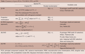
Here we discuss three types of sparse PCA which are divided into four different approaches. The three types are variance maximization (VM), projection minimization, and probabilistic model (PM). All of them can be used to derive PCA. To achieve sparseness, the L1-penalty function is added in the PCA estimation process. A summary is given in Table 1.
Full table
Variance maximization (VM) approach
The approach aims to project data points into a low-dimensional space (data reduction) with a goal to preserve their variation of original samples points as much as possible.
Mathematically, assume that X represents original data (a n samples by p variables matrix), the corresponding first loading coefficient vector is , and the corresponding PC is. Maximization of the variance of can be expressed by the form:
By imposing a L1-penalty function (, where is the absolute value) in the Eq. [1], it becomes a sparse PCA:
The, is a penalty parameter that controls the amount of shrinkage on each PC. The larger the value of λj, the greater the amount of shrinkage (i.e. the greater the amount of zero estimates). Algorithm to implement the VM includes Trendafilov and Jolliffe (34) and Croux, Filzmoser (35) with an available R package, pcaPP.
Projection minimization is another way to compute PCA. The method targets the minimum distant between the projected data and the observed data. Thus, PCA can be alternatively modeled as the following formulation where V is the loading coefficient matrix.
Two strategies are evaluated here to perform sparseness while conducting projection minimization for PCA.
Reconstruction error minimization (REM)
Zou and Hastie (22) reconstructed the product of the loading coefficient matrix, , into two matrices (A, B) and add a L2-norm penalty on B, so the formulation of PCA becomes
where A and B are both p×k matrix, and λ is the penalty parameter. The solution of B is equivalent to the ridge regression problem, and then the loading is .
To impose sparseness, a L1-norm penalty on B is added to obtain sparse loadings, and the formula becomes
whereas a common λ is used for all PCs, but different are allowed for penalizing the loadings of different PCs. This approach can be expressed in another way by performing alternating estimation for the solution of Eq. [5], i.e., estimate one of parameter when the other is fixed. In other words, estimating B given A is the elastic net regression estimation (36); on the other hand, estimating A given B is a reduced rank Procrustes rotation problem. A R package, elasticnet, is available to perform the REM (22).
Singular value decomposition (SVD)
Another way to reconstruct the product of the loading coefficient matrix, , is to use SVD to extract the PCs through solving a low rank matrix approximation problem. Mathematically, let the SVD of X be , where U is an n by k orthogonal matrix, U is an p by k orthogonal matrix, and D is a k by k diagonal matrix and assumed to be ordered so that. Consequently, the estimation of U, D, and V can be formulated as the following optimization problem:
Shen and Huang (24) introduced a L1-norm penalty in Eq. [6], to promote sparse loadings, and the penalized mathematical formula becomes
where λj is the penalty parameter for each component. There are two R functions available to this sparse PCA. One is PMD R package using cross validation (CV) to determine the penalty parameter (26). The other is a R code (https://www.unc.edu/~haipeng) using Bayesian information criterion (BIC) to select the penalty parameter value (24).
Probabilistic modeling (PM)
PCA can be also reformulated as a maximum likelihood solution to a latent variable model, called probabilistic PCA (37). The PM for PCA is represented by
where Z is PCs whose row vector is consider as an k-dimensional latent variables, λ is the noisy, and both the latent variable and noise are assumed to be isotropic normal distribution, . Then, the marginal distribution of X is normal distribution with zero means and covariance, V'V+σ2Ip. Estimation of the parameters V and σ2 can be done by the maximum-likelihood function.
To perform sparseness on loading coefficients, we can assign Laplacian prior to each element of loadings in the PM [the Laplacian prior is equivalent to L1 regularization in the sparse modeling (38)]. The resulting sparse probabilistic PCA is to estimate the following parameters
The Bayesian solution, such as variational expectation-maximization (EM) algorithm (27,39) or Markov Chain Monte Carlo algorithm (40), can be used to estimate the parameters. A R package, nsprcomp, is available to run this approach (39).
Finally, the performance of sparse loading depends on the penalty parameters , because the determines the degree of sparseness of loadings. Usually, selecting the optimal values of can use cross-validation (CV) or BIC: CV is to choose a set of penalty parameters such that there is a minimum prediction error when we divide the samples into testing and training dataset, and use the estimates of training dataset to predict testing dataset; BIC composes of the measurement of estimation error and the degree of freedom of model. The estimation error is the distant between the data and estimates, and Zou, Hastie (41) has shown that the degree of freedom of lasso is the number of non-zero coefficients.
Simulation
Approaches for comparison
A simulation study is conducted to compare the performance of the four sparse PCA approaches and the classic PCA: (I) VM using the R package, pcaPP; (II) REM using the R package, elasticnet; (III) SVD: two algorithms are considered: one with BIC (SVDb), and the other with CV (SVDc) using the R package, PDM; (IV) PM using the R package, nsprcomp.
Design
The simulated data, X, is generated from normal distribution with zero mean and covariance, , where the sample size is fixed by 100, V is a p×3 orthogonal matrix (including three PCs sorted by eigen-value), is an identity matrix.
We consider two cases: one with the numbers of variables less than the sample size: 50 (n>p). The other is the numbers of variables greater than the sample size: 300 (p>n). In addition, we discuss two different covariance structures to compare the performance in dealing the orthogonality constraint: (I) non-overlap structure (Figure 1A): the first 10 variables are assigned to first component with a uniform loading coefficient value, 0.32, the 11th-20th variables are assigned with a uniform loading coefficient value, 0.32, to second component, the 21th-30th variables are assigned to third component with a uniform loading coefficient value, 0.32. The remaining variables are given a zero value for the loading coefficients (i.e. three vectors of loading are non-overlap); (II) overlap structure (Figure 1B): the first 15 variables are assigned to first component [loading coefficient value = (0.256,…,0.256)], the 6th-25th variables are assigned to second component [loading coefficient value = (0.132, –0.061, –0.061, –0.061, 0.061, 0.022, …, 0.022, 0.310,…)], the 16th-35th variables are assigned to third component (loading coefficient value = (–0.2842, –0.0711, –0.0711, –0.0711, 0.0995, …, 0.0995, 0.292, …), the other variables are given a zero value for the loading coefficients (i.e. three vectors of loading are overlap).
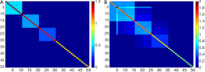
Therefore, there are four simulated cases: (I) non-overlap covariance structure with p=50; (II) non-overlap covariance structure with p=300; (III) overlap covariance structure with p=50; (IV) non-overlap covariance structure with p=300, respectively.
The simulations are replicated by 300 times for each case and the first three PCs are evaluated.
Metric for comparison
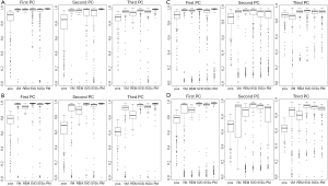
A consistency metric, cosine value of the angle between the true and the estimated vector of sparse loading coefficients, is used as the performance indicator. The cosine value in each replication is defined as the inner product of true and estimated loading coefficients. Like the correlation coefficient (but in a range of 0 and 1), if the estimated loading coefficients are very close to the true loading coefficients, then the cosine value will be approximate to 1 (the angle of true and estimated loading coefficients is close to 0). In contrast, if the estimated loading coefficients are quite different from the true loading coefficients, then the cosine value will approach to 0 (the angle of true and estimated loading coefficients is close to 90). The cosine values of 300 replications in each algorithm are presented by boxplot (Figure 2).
Results
Results of the four simulation studies are presented in Figure 2A-D. Clearly, all sparse PCAs perform well with high consistency (>90%) compared to the classic PCA with a consistency rate <80% in most cases (Figure 2A-D). This indicates the sparse PCAs could predict well the true loading coefficient values. In comparison of non-overlap versus overlap structure, sparse PCAs perform better in the case with non-overlap structure (Figure 2A-B versus 2C-D). In addition, higher consistency rate is observed in PC1 than in PC2 or PC3 for the sparse PCAs (Figure 2A-D). Also, sparse PCAs perform better when the number of genes is smaller (Figure 2A versus 2B or 2C versus 2D).
Data example
To illustrate the potential application of sparse PCA, a gene expression dataset in lung cancer (n=442 patients) is used for demonstration (42). In this dataset, there are 255 patients survived more than 5 years (censored at 5 years) and 187 patients died before 5 years. Demographic information includes gender (female: 219, male: 223), smoking status (never smoking: 49, past smoking: 268, and current smoking: 32), and TNM staging (IA: 114, IB: 162, II: 95; III: 68). Here we used one published gene signature, malignancy risk (MR) gene signature (102 genes) (7), to evaluate if any sparse PCA could perform better than the classic PCA in terms of reduction of gene numbers and improvement of difference of survival curves. The analysis procedures is first to reduce the data into PC1, then to divide the 442 patients into two risk groups (high and low malignancy-risk groups) according to a zero split of the PC1, and lastly to use Kaplan Meier method to estimate survival curve for each group and log rank-test to test significant difference of two survival curves.
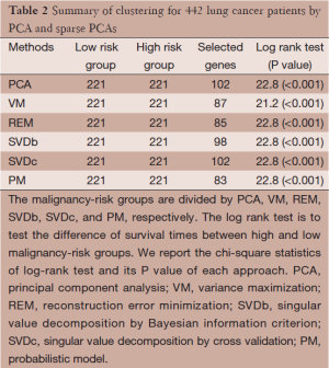
Analysis results are presented in Table 2 for the comparison of PCA with sparse PCAs, including VM, REM, SVD, and PM approaches. Each approach is able to show a statistically significant difference between the two survival curves (P<0.001). Ideally, we would like to the sparse PCAs yields a smaller subset of genes with a larger chi-square statistics of log rank test (i.e., smaller P value). While the results show a comparable chi-square statistics (21.2-22.8; P<0.001), some of sparse PCA approaches (e.g., REM and PM) select fewer genes to more efficiently contribute to the risk classification.
Full table
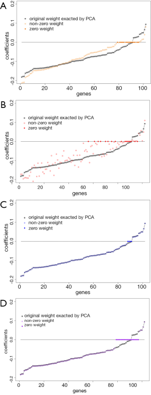
To illustrate how the sparse PCAs shrink the loading coefficients to zero, we compare the loading coefficients between each sparse PCA and the classic PCA in Figure 3. Results indicate if the loading coefficients in the classic PCA are close to zero, they are likely to be shrunken to zero by spare PCA.
Conclusions
Sparse PCA is a modern advanced PCA by maintaining the powerful data reduction functionality and incorporating the sparseness model for variable selection. While its application in cancer research is still in infancy stage compared to PCA, we see the great potential especially in the some cancer types (e.g., pancreatic cancer) which gene expression levels are quite homogeneous, and thus make very challenging to develop genomic profiles.
Acknowledgments
We are grateful to the reviewers for their constructive comments which led to improvements in this manuscript.
Funding: The study was supported in part by Taiwan National Science Council (NSC 101-2118-M-005-002 to Y-L.H. and Graduate Students Study Abroad Program to P-Y.H.) and the National Institutes of Health (5P30CA076292 to D-T.C.).
Footnote
Provenance and Peer Review: This article was commissioned by the editorial office, Translational Cancer Research for the series “Statistical and Bioinformatics Applications in Biomedical Omics Research”. The article has undergone external peer review.
Conflicts of Interest: All authors have completed the ICMJE uniform disclosure form (available at http://dx.doi.org/10.3978/j.issn.2218-676X.2014.05.06). The series “Statistical and Bioinformatics Applications in Biomedical Omics Research” was commissioned by the editorial office without any funding or sponsorship. DTC served as the unpaid Guest Editor of the series and serves as an unpaid editorial board member of Translational Cancer Research. The authors have no other conflicts of interest to declare.
Ethical Statement: The authors are accountable for all aspects of the work in ensuring that questions related to the accuracy or integrity of any part of the work are appropriately investigated and resolved.
Open Access Statement: This is an Open Access article distributed in accordance with the Creative Commons Attribution-NonCommercial-NoDerivs 4.0 International License (CC BY-NC-ND 4.0), which permits the non-commercial replication and distribution of the article with the strict proviso that no changes or edits are made and the original work is properly cited (including links to both the formal publication through the relevant DOI and the license). See: https://creativecommons.org/licenses/by-nc-nd/4.0/.
References
- Chen DT, Nasir A, Culhane A, et al. Proliferative genes dominate malignancy-risk gene signature in histologically-normal breast tissue. Breast Cancer Res Treat 2010;119:335-46. [PubMed]
- Seierstad T, Røe K, Sitter B, et al. Principal component analysis for the comparison of metabolic profiles from human rectal cancer biopsies and colorectal xenografts using high-resolution magic angle spinning 1H magnetic resonance spectroscopy. Mol Cancer 2008;7:33. [PubMed]
- Khan J, Wei JS, Ringnér M, et al. Classification and diagnostic prediction of cancers using gene expression profiling and artificial neural networks. Nat Med 2001;7:673-9. [PubMed]
- Hunter DJ, Kraft P, Jacobs KB, et al. A genome-wide association study identifies alleles in FGFR2 associated with risk of sporadic postmenopausal breast cancer. Nat Genet 2007;39:870-4. [PubMed]
- Price AL, Patterson NJ, Plenge RM, et al. Principal components analysis corrects for stratification in genome-wide association studies. Nat Genet 2006;38:904-9. [PubMed]
- Pomeroy SL, Tamayo P, Gaasenbeek M, et al. Prediction of central nervous system embryonal tumour outcome based on gene expression. Nature 2002;415:436-42. [PubMed]
- Chen DT, Hsu YL, Fulp WJ, et al. Prognostic and predictive value of a malignancy-risk gene signature in early-stage non–small cell lung cancer. J Natl Cancer Inst 2011;103:1859-70. [PubMed]
- Wigle DA, Jurisica I, Radulovich N, et al. Molecular profiling of non-small cell lung cancer and correlation with disease-free survival. Cancer Res 2002;62:3005-8. [PubMed]
- Larsen JE, Pavey SJ, Passmore LH, et al. Gene expression signature predicts recurrence in lung adenocarcinoma. Clin Cancer Res 2007;13:2946-54. [PubMed]
- Raponi M, Zhang Y, Yu J, et al. Gene expression signatures for predicting prognosis of squamous cell and adenocarcinomas of the lung. Cancer Res 2006;66:7466-72. [PubMed]
- Kratz JR, Jablons DM. Genomic prognostic models in early-stage lung cancer. Clin Lung Cancer 2009;10:151-7. [PubMed]
- Boutros PC, Lau SK, Pintilie M, et al. Prognostic gene signatures for non-small-cell lung cancer. Proc Natl Acad Sci U S A 2009;106:2824-8. [PubMed]
- Roepman P, Jassem J, Smit EF, et al. An immune response enriched 72-gene prognostic profile for early-stage non-small-cell lung cancer. Clin Cancer Res 2009;15:284-90. [PubMed]
- Li J, Szekely L, Eriksson L, et al. High-throughput mammographic-density measurement: a tool for risk prediction of breast cancer. Breast Cancer Res 2012;14:R114. [PubMed]
- Navarro Silvera SA, Mayne ST, Risch HA, et al. Principal component analysis of dietary and lifestyle patterns in relation to risk of subtypes of esophageal and gastric cancer. Ann Epidemiol 2011;21:543-50. [PubMed]
- Hausman R. Constrained multivariate analysis. Optimisation in Statistics 1982:137-51.
- Vines S. Simple principal components. J R Stat Soc Ser C Appl Stat 2000;49:441-51.
- Cadima J, Jolliffe IT. Loading and correlations in the interpretation of principle compenents. J Appl Stat 1995;22:203-14.
- Al-Kandari NM, Jolliffe IT. Variable selection and interpretation in correlation principal components. Environmetrics 2005;16:659-72.
- Jolliffe IT. Rotation of principal components: choice of normalization constraints. J Appl Stat 1995;22:29-35.
- Tibshirani R. Regression shrinkage and selection via the lasso. J R Stat Soc Series B Stat Methodol 1996;58:267-88.
- Zou H, Hastie T, Tibshirani R. Sparse principal component analysis. J Comput Graph Stat 2006;15:265-86.
- Jolliffe IT, Trendafilov NT, Uddin M. A modified principal component technique based on the LASSO. J Comput Graph Stat 2003;12:531-47.
- Shen H, Huang JZ. Sparse principal component analysis via regularized low rank matrix approximation. J Multivar Anal 2008;99:1015-34.
- d’Aspremont A, El Ghaoui L, Jordan MI, et al. eds. A direct formulation for sparse PCA using semidefinite programming. NIPS, 2004.
- Witten DM, Tibshirani R, Hastie T. A penalized matrix decomposition, with applications to sparse principal components and canonical correlation analysis. Biostatistics 2009;10:515-34. [PubMed]
- Guan Y, Dy JG, eds. Sparse probabilistic principal component analysis. International Conference on Artificial Intelligence and Statistics, 2009.
- Bernardo J, Bayarri M, Berger J, et al. Bayesian factor regression models in the “large p, small n” paradigm. Bayesian Statistics 2003;7:733-42.
- Carvalho CM, Chang J, Lucas JE, et al. High-Dimensional Sparse Factor Modeling: Applications in Gene Expression Genomics. J Am Stat Assoc 2008;103:1438-56. [PubMed]
- Lee M, Shen H, Huang JZ, et al. Biclustering via sparse singular value decomposition. Biometrics 2010;66:1087-95. [PubMed]
- Yang D, Ma Z, Buja A. A sparse SVD method for high-dimensional data. J Comput Graph Stat 2013; [Crossref]
- Sill M, Kaiser S, Benner A, et al. Robust biclustering by sparse singular value decomposition incorporating stability selection. Bioinformatics 2011;27:2089-97. [PubMed]
- Bi J, Bennett K, Embrechts M, et al. Dimensionality reduction via sparse support vector machines. The Journal of Machine Learning Research. 2003;3:1229-43.
- Trendafilov NT, Jolliffe IT. Projected gradient approach to the numerical solution of the SCoTLASS. Comput Stat Data Anal 2006;50:242-53.
- Croux C, Filzmoser P, Fritz H. Robust sparse principal component analysis. Technometrics 2013;55:202-14.
- Zou H, Hastie T. Regularization and variable selection via the elastic net. J R Stat Soc Series B Stat Methodol 2005;67:301-20.
- Tipping ME, Bishop CM. Probabilistic principal component analysis. J R Stat Soc Series B Stat Methodol 1999;61:611-22.
- Williams PM. Bayesian regularization and pruning using a Laplace prior. Neural Comput 1995;7:117-43.
- Sigg CD, Buhmann JM. eds. Expectation-maximization for sparse and non-negative PCA. Proceedings of the 25th international conference on Machine learning, 2008:ACM.
- Mohamed L, Calderhead B, Filippone M, et al. Population MCMC methods for history matching and uncertainty quantification. Comput Geosci 2012;16:423-36.
- Zou H, Hastie T, Tibshirani R. On the “degrees of freedom” of the lasso. Ann Stat 2007;35:2173-92.
- Shedden K, Taylor JM, Enkemann SA, et al. Gene expression-based survival prediction in lung adenocarcinoma: a multi-site, blinded validation study. Nat Med 2008;14:822-7. [PubMed]


